Recently, I’ve been reading a book and watching a lecture series about model checking. This is a topic I’ve learned a bit about in the past, but never really studied in earnest. I highly recommend these resources to anyone who is interested in learning more.

In model checking, we create a model of some sort of stateful artifact, like a computer program, sequential circuit, or even something in the “real world” (like a vending machine or traffic light). Then, we state a property we would like to hold about all possible behaviors of the model. Finally, we check whether this property holds for the model, using a variety of nifty algorithms.

This series of blog posts constitutes a straightforward introduction to model checking, using Haskell code to express the ideas and implement the algorithms. The intended audience is anyone who knows a bit of Haskell and a bit of logic, and who wants to understand how model checking works.

This post was generated with pandoc from a literate haskell document.

What is model checking?

Modern physical and digital systems can be incredibly complex. They are often composed of multiple interacting subsystems, each with its own internal state. It can become extremely hard to reason about the correctness of these systems, because the details of exactly how and when the system changes state may be subtle.

There is only one way to get hard guarantees about a complex system: by using mathematical rigor to describe the system in question, to specify the desired property, and to prove or disprove that the system satisfies the property. This can be done entirely manually (i.e. constructing a proof or counterexample by hand), or with the help of some degree of tool automation. Typically, the more automation a technique offers, the more limited it is in other aspects (for instance, in the size of the models that can be verified). Hand proofs, automated theorem proving, abstract interpretation, SAT/SMT solving, BDDs, and model checking are all examples of formal methods techniques, and each of these techniques occupies its own special compromise point in the design space.

Model checking is at the “high automation/limited scalability” end of this spectrum. Model checking is extremely powerful because it is a push-button process. Once you specify your model and the property you want to check, the computer does the rest. However, the method is fundamentally limited by the “state-explosion” problem. Model checking involves an exhaustive search of the entire state space of a system, and if this space is too big, verification becomes infeasible. Model checking has had most of its success in the hardware domain, where state and control logic are much smaller and simpler than in a typical piece of software. It is a good method to use for finding bugs because it’s great at producing small counterexamples, if they exist.

In practice, model checking consists of three basic steps:

1. Capture the essence of the system you want to verify by constructing a model of this system, using a formal language that a model checking tool can understand.

2. Capture the property you want to verify about your model in a property specification language (usually this is the same language in which the model is described).

3. Press “go”, and wait for the tool to either a) declare that the property holds for your model, b) provide a counterexample, or c) give up.

The basic idea of model checking is simple: represent all possible states of your system as nodes in a directed graph, and represent the possible changes from state to state as directed edges from one node to another. Then, checking a property of your system boils down to running some sort of search algorithm on the graph. This graph-based representation is called a transition system.

The goal of this first post is to introduce the notion of a transition system, and to show how we can verify a simple type of property called an invariant. The example used throughout this post (a traffic light with three states) is a pedagogical one, and it’s very trivial. The point in this first post is not to show you the full power of model checking all at once; it’s to set up a conceptual framework that we can build on in subsequent posts.

Each post will build on the previous one, and we will gradually move from simple systems and properties to more complex and meaningful ones. By the final post in this series, we will have developed a full-blown model checker in Haskell, and we will use it to verify some non-trivial properties about a cache coherence protocol.

Transition systems

module ModelChecking1 where

import Data.List (find)
import System.Random (RandomGen, randomR)

A transition system over state set s, action set action, and atomic propositional variables ap is defined as follows:

data TransitionSystem s action ap = TransitionSystem
  { tsInitialStates :: [s]
  , tsLabel         :: s -> [ap]
  , tsTransitions   :: s -> [(action, s)]
  }

The type s represents all possible states our system can be in; if the system is a traffic light, s might be the set of colors {red, green, yellow}; if it’s a sequential circuit, it might be the current value of a set of bits.

The type ap represents the relevant properties of a given state. Depending on what property we are interested in for our system, we might choose a corresponding set of variables ap that help us to capture the property using propositional logic. Each element of ap is a boolean-valued variable, and depending on which state the system is in, each such variable may be either true or false. The tsLabel function tells us the true-set of each state. The true-set is simply the set of variables which are true in a given state. If a variable is in this list, then it’s true; if it’s absent from the list, it’s false.

The type action is simply a “name” for each outgoing transition. These names do not carry any semantic content, but it’s often useful to give a name to a transition to indicate “what is happening” as the system changes from state to another.

In summary, here is the intuition behind each of the three fields of a transition system.

• tsInitialStates ts: “the states that the system can start in”
• tsLabel ts s: “the set of variables which are true in state s”
• tsTransitions ts s: “all of s’s outgoing transitions”

Let’s look at a trivial example of a transition system.

Example: Traffic light

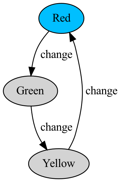
We can create a very simple transition system representing the states and transitions of a traffic light. The states s will be the colors red, yellow, and green:

data Color = Red | Yellow | Green deriving (Show, Eq, Ord)

The atomic propositional variables ap that we will use is also Color. The idea is that a color is True in a given state if and only if that color is currently lit up. In this example, states and atomic propositional variables are one and the same; however, this will not always be the case, and when we study more interesting examples, we will use a much richer set of atomic propositional variables.

There will only be one action:

data Change = Change deriving (Show, Eq, Ord)

Our set of transitions will allow Red to transition to Green, Green to Yellow, and Yellow to Red. Below is the definition of the traffic light’s transition system:

traffic_light :: TransitionSystem Color Change Color
traffic_light = TransitionSystem
  { tsInitialStates = [Red]
  , tsLabel = \s -> [s]
  , tsTransitions = \s -> case s of
      Red    -> [(Change, Green )]
      Green  -> [(Change, Yellow)]
      Yellow -> [(Change, Red   )]
  }

Notice that in each state s, where s is one of the colors Red, Yellow, or Green, the label of s is simply [s], because the only color that is lit up in state s is s itself.

Running a transition system

A run of a transition system is a finite or infinite path in the underlying graph:

data Path s action = Path { pathHead :: s, pathTail :: [(action, s)] }
  deriving (Show)

The following path-constructing functions will be useful:

singletonPath :: s -> Path s action
singletonPath s = Path s []

consPath :: (s, action) -> Path s action -> Path s action
consPath (s, action) (Path s' tl) = Path s ((action, s'):tl)

reversePath :: Path s action -> Path s action
reversePath (Path s prefix) = go [] s prefix
  where go suffix s [] = Path s suffix
        go suffix s ((action, s'):prefix) = go ((action, s):suffix) s' prefix

In the transitions systems we’ll define, it will be useful to be able to examine random infinite runs of the system to get a feel for what the possibilites are:

randomRun :: RandomGen g => g -> TransitionSystem s action ap -> Path s action
randomRun g ts = let (i, g') = randomR (0, length (tsInitialStates ts) - 1) g
                     s = tsInitialStates ts !! i
                 in Path s (loop g' s ts)
  where loop g s ts = let nexts = tsTransitions ts s
                          (i, g') = randomR (0, length nexts - 1) g
                          (action, s') = nexts !! i
                      in (action, s') : loop g' s' ts

Let’s generate a random run of our traffic_light example in ghci:

  > import System.Random
  > g = mkStdGen 0
  > r = randomRun g traffic_light
  > pathHead r
  Red
  > take 6 (pathTail r)
  [(Change,Green),(Change,Yellow),(Change,Red),(Change,Green),(Change,Yellow),(Change,Red)]

Because each state in traffic_light has exactly one outgoing transition, this is the only run we will ever get. In subsequent posts, we’ll look at nondeterministic transition systems which will return different runs with different random generators.

Checking invariants

Given a state s of a transition system ts, we can ask which atomic propositional variables hold in s; that is, given a particular variable p :: ap, we can determine whether p is true in s via

p `elem` tsLabel ts s

If the result of this call is True, then p is True in state s; if it is False, then p is False in state s.

We can generalize this from atomic propositional variables to all propositions, which are logical formulas stated “in terms of” the variables ap, using boolean connectives (and, or, implies, not) to build larger formulas out of smaller ones. In this section, will define a Proposition in Haskell to be any function that maps true-sets to Bools. Since the label of every state in a transition system is its true-set, we can therefore ask, for each individual state, whether a given proposition is true when evaluated at the label of that state – that is, whether the state satisfies the proposition.

We can take this one step further and ask whether a proposition is satisfied by every reachable state of a transition system. If this is true for a given proposition, that proposition is said to be an invariant of the system. In order to determine whether a given proposition is an invariant, we simply search the transition system’s underlying graph, evaluating the proposition at every state label we reach; if any of the labels do not satisfy the proposition, then it is not an invariant.

This section will introduce the definition of a Proposition, and will define a simple depth-first search function over a transition system that checks whether a given proposition holds for all reachable states of the system. We will then apply this function to our traffic light system to check that a very simple invariant holds.

Predicates

In this section, we’ll introduce the general notion of a predicate, which we will use in this post and in every subsequent post. We will see that a proposition is a special type of predicate.

A predicate is any single-argument function that returns a Bool:

type Predicate a = a -> Bool

Predicates are a fundamental building block for many of the most commonly used functions in Haskell:

even   :: Integral a => Predicate a
null   :: Foldable t => Predicate (t a)
and    :: Foldable t => Predicate (t Bool)
all    :: Foldable t => Predicate a -> Predicate (t a)
filter :: Predicate a -> [a] -> [a]

A very simple example of a predicate is true, which holds for all inputs:

true :: Predicate a
true _ = True

Similarly, false holds for no inputs:

false :: Predicate a
false _ = False

We can “lift” all of the usual boolean operators to work with predicates:

(.&) :: Predicate a -> Predicate a -> Predicate a
(p .& q) a = p a && q a
infixr 3 .&

(.|) :: Predicate a -> Predicate a -> Predicate a
(p .| q) a = p a || q a
infixr 2 .|

pnot :: Predicate a -> Predicate a
pnot p a = not (p a)

(.->) :: Predicate a -> Predicate a -> Predicate a
(p .-> q) a = if p a then q a else True
infixr 1 .->

These operators (called boolean connectives) are useful for building larger predicates out of smaller ones:

  > divisible_by_3 a = a `mod` 3 == 0
  > divisible_by_6 = even .& divisible_by_3
  > map divisible_by_6 [0..12]
  [True,False,False,False,False,False,True,False,False,False,False,False,True]

When working with predicates, the following “flipped application” operator is useful:

(|=) :: a -> Predicate a -> Bool
a |= p = p a
infix 0 |=

Given some object a, and some predicate p :: Predicate a, we read the statement a |= p as “a satisfies p”.

  > 5 |= divisible_by_6     -- Does 5 satisfy divisible_by_6?
  False
  > [2, 10, 24] |= all even -- Does [2, 10, 24] satisfy all even?
  True

This flipped application syntax may seem weird, but reading |= as “satisfies” should help.

Propositions

We define a proposition over the atomic propositions ap to be a predicate over [ap]:

type Proposition ap = Predicate [ap]

In this context, a list aps :: [ap] is thought of as “the set of all atomic propositions which are true.” Given a single atomic proposition p, we can form the proposition “p holds” as follows:

atom :: Eq ap => ap -> Proposition ap
atom p aps = p `elem` aps

Using the atom function, along with our boolean connectives .&, .|, .->, and pnot, we can “build up” propositional formulas from atomic propositions, and we can then ask whether the resulting formula is satisfied by a particular true-set. Let’s mess around a bit in ghci to get a feel for how this works:

  > data AB = A | B deriving (Show, Eq)
  > [A] |= atom A
  True
  > [A] |= atom B
  False
  > [A] |= pnot (atom B)
  True
  > [A] |= atom A .& atom B
  False
  > [A] |= atom A .| atom B
  True
  > [A] |= atom A .-> atom B
  False
  > [A] |= atom B .-> atom A
  True

Recall that our states are labeled by true-sets:

tsLabel :: TransitionSystem s action ap -> s -> [ap]

Therefore, given a proposition f :: Proposition ap, which is just a function f :: [ap] -> Bool, we can ask whether a particular state s of our transition system satisfies f like so:

tsLabel ts s |= f

Let’s try this out a bit with our traffic light system:

  > tsLabel traffic_light Red -- which colors are "true" in state Red?
  [Red]
  > tsLabel traffic_light Red |= atom Red
  True
  > tsLabel traffic_light Red |= (atom Red .| atom Green)
  True
  > tsLabel traffic_light Red |= atom Red .-> atom Yellow
  False
  > tsLabel traffic_light Red |= atom Yellow .-> atom Green
  True

Depth-first search

Given a transition system ts and a proposition f over ts’s atomic propositional variables, we can ask: “Does f hold at all reachable states in ts?” A proposition which is supposed to hold at all reachable states of a transition system is called an invariant.

To check whether an invariant holds, we evaluate the proposition on each reachable state (more precisely, on the label of each reachable state). To do this, we first define a lazy depth-first search to collect all the states.

Our depth-first search algorithm produces each reachable state, along with the path traversed to reach that state. The path will be useful for giving informative counterexamples.

dfs :: Eq s => [s] -> (s -> [(action, s)]) -> [(s, Path s action)]
dfs starts transitions = (\p@(Path s tl) -> (s, reversePath p)) <$> loop [] (singletonPath <$> starts)
  where loop visited stack = case stack of
          [] -> []
          ((Path s _):stack') | s `elem` visited -> loop visited stack'
          (p@(Path s _):stack') ->
            let nexts = [ consPath (s', action) p | (action, s') <- transitions s ]
            in p : loop (s:visited) (nexts ++ stack')

The checkInvariant function

Now, to check whether a proposition f :: Proposition ap is an invariant of a transition system, we simply collect all the system’s reachable states via dfs and make sure the invariant holds for each of their labels, producing a path to a bad state if there is one:

checkInvariant :: Eq s
               => Proposition ap
               -> TransitionSystem s action ap
               -> Maybe (s, Path s action)
checkInvariant f ts =
  let rs = dfs (tsInitialStates ts) (tsTransitions ts)
  in find (\(s,_) -> tsLabel ts s |= pnot f) rs

Checking a traffic light invariant

Let’s check an invariant of our traffic light system – that the light is never red and green at the same time. It’s not a very interesting invariant, but it’s a good one for any traffic light to have.

  > checkInvariant (pnot (atom Red .& atom Green)) traffic_light
  Nothing

The result Nothing means there were no counterexamples, which means our invariant holds! Let’s try it with an invariant that doesn’t hold:

  > checkInvariant (pnot (atom Yellow)) traffic_light
  Just (Yellow,Path {pathHead = Red, pathTail = [(Change,Green),(Change,Yellow)]})

Our invariant checking algorithm was able to find a path to a state that violated pnot (atom Yellow); unsurprisingly, the bad state was Yellow. Because Yellow is reachable in our transition system, this property doesn’t hold. What if, however, Yellow is not reachable – for instance, in a simpler traffic light that goes directly from Green to Red?

simple_traffic_light :: TransitionSystem Color Change Color
simple_traffic_light = TransitionSystem
  { tsInitialStates = [Red]
  , tsLabel = \s -> [s]
  , tsTransitions = \s -> case s of
      Red   -> [(Change, Green)]
      Green -> [(Change, Red  )]
  }

If we check pnot (atom Yellow), we will find that the property holds, because Yellow isn’t reachable:

  > checkInvariant (pnot (atom Yellow)) simple_traffic_light
  Nothing

What’s next?

This post describes the basic idea of model checking: represent the system you’d like to verify as a directed graph, and search the graph to make sure the desired property holds. The system we studied was simple enough to be pedagogically useful, but might be too trivial to illustrate the power of the technique. Furthermore, the property we verified was also extremely simple.

In the next post, we’ll discuss a technique for converting imperative computer programs into transition systems, and we will use this technique to verify a non-trivial invariant about a non-trivial program. In the post after that, we’ll discuss how to state and verify more interesting properties, like “every red light is immediately preceded by a yellow light.”